6장 연습문제 : 국내 총생산 vs 알코올 소비량
문제 내용
위키피디아에는 1인당 알코올 소비량과 국가별 1인당 국내 총생산 등 다양한 인구통계 데이터가 들어있다. 이 데이터를 사용해서 GDP 기준(평균 이상 vs 평균 이하)과 알코올 소비량 기준(평균 이상 vs 평균 이하)으로 교차 집계하는 프로그램을 짜 보자. 두 기준이 서로 연관되어 있는지 판단해보자.
GDP 자료 : goo.gl/RUiLoa 알코올 소비량 자료 : goo.gl/qZZvNg
자료 만들기
- 일단 바로 다운로드할 수 있는 방법은 없는 것 같아 필요한 자료를 복사해 엑셀에 붙여넣고 CSV 파일로 생성
- Pandas로 읽어와 데이터 프레임으로 만든다.
import pandas as pd
import numpy as np

gdp = pd.read_csv("gdp.csv")
alco = pd.read_csv("alchol.csv")

gdp.info()
'''출력
<class 'pandas.core.frame.DataFrame'>
RangeIndex: 196 entries, 0 to 195
Data columns (total 3 columns):
 #   Column             Non-Null Count  Dtype
---  ------             --------------  -----
 0   Rank               196 non-null    object
 1   Country/Territory  196 non-null    object
 2   Int$               196 non-null    object
dtypes: object(3)
memory usage: 4.7+ KB
'''

alco.info()
'''출력
<class 'pandas.core.frame.DataFrame'>
RangeIndex: 189 entries, 0 to 188
Data columns (total 10 columns):
 #   Column                  Non-Null Count  Dtype
---  ------                  --------------  -----
 0   Country                 189 non-null    object
 1   Total                   189 non-null    float64
 2   Recorded consumption    189 non-null    float64
 3   Unrecorded consumption  189 non-null    float64
 4   Beer(%)                 179 non-null    float64
 5   Wine(%)                 179 non-null    float64
 6   Spirits(%)              179 non-null    float64
 7   Other(%)                179 non-null    float64
 8   2020 projection         189 non-null    float64
 9   2025 projection         188 non-null    float64
dtypes: float64(9), object(1)
memory usage: 14.9+ KB
'''
- GDP.csv에 포함된 GDP 금액 값에 ,가 포함되어 있고 수치형 데이터가 아니므로 이를 처리해준다.
# GDP 컬럼의 값들에 포함된 , 제거
gdp["Int$"] = gdp["Int$"].str.replace(',', '')

# 수치형으로 변환
gdp["Int$"] = pd.to_numeric(gdp["Int$"], errors='coerce')

gdp["Int$"].info()
'''출력
<class 'pandas.core.frame.DataFrame'>
RangeIndex: 196 entries, 0 to 195
Data columns (total 3 columns):
 #   Column             Non-Null Count  Dtype
---  ------             --------------  -----
 0   Rank               196 non-null    object
 1   Country/Territory  196 non-null    object
 2   Int$               196 non-null    int64
dtypes: int64(1), object(2)
memory usage: 4.7+ KB
'''
- GDP 데이터에 평균값을 기준으로 평균 초과 vs 평균 이하를 구분하는 값을 가진 컬럼을 추가해준다.
gdp_mean = gdp["Int$"].mean()
gdp_mean
'''출력
21701.367346938776
'''

# 각각의 GDP를 GDP 평균(gdp_mean)과 비교하여 평균보다 크면 1을 평균 이하이면 0을 리턴한다.
# 이렇게 만들어진 컬럼을 gdp 데이터프레임에 추가한다.

def mean_division (x, mean) :
    if x > mean:
        return 1
    return 0

gdp["Mean Division"] = gdp["Int$"].apply(lambda x: mean_division(x, gdp_mean))

# 컬럼 이름도 바꿔주자
gdp.columns = ["Rank", "Country", "GDP", "Mean Division(GDP)"]
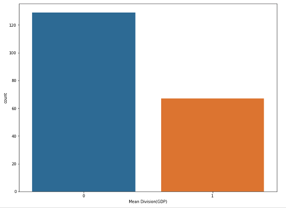
- GDP 데이터를 평균 기준으로 나눈 자료를 그래프로 표시해보자. seaborn을 사용했다.
import matplotlib.pyplot as plt
import seaborn as sns

plt.rcParams["figure.figsize"] = (12, 9)
sns.countplot(x="Mean Division(GDP)", data=gdp)
- 알코올 데이터는 수치형 데이터로 되어있기는 하지만 결측값이 있다. 임의의 값을 넣기는 좀 그러니 행을 제거해버리자.
# 결측치가 있는 행 모두 삭제 처리
alco.dropna()
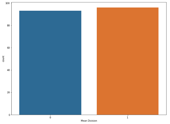
- 평균을 구하고 편균을 기준으로 구분한 구분자 컬럼을 추가하고 그래프를 그리는 것 까지 이전과 동일하다.
alco_mean = alco["Total"].mean()

alco["Mean Division"] = alco["Total"].apply(lambda x: mean_division(x, alco_mean))

sns.countplot(x="Mean Division", data=alco)
- 이제 국가명을 기준으로 두 데이터 프레임을 합쳐보자.
merged_df = pd.merge(gdp, alco, how="outer", on="Country")
- 마지막으로 GDP 기준 그래프에 알코올 소비량이 비교되도록 그래프를 그려보자
sns.countplot(x="Mean Division(GDP)", hue="Mean Division", data=merged_df)
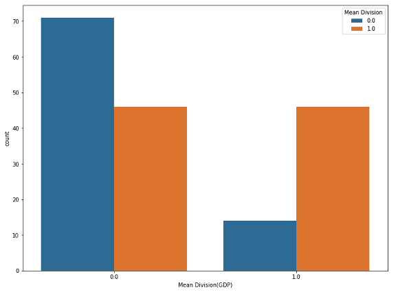
제대로 한 건가 모르겠다…-.-